ML Sketching

Last updated Feb 28, 2025 Edit Source

• Houdini
• Machinelearning

This is one of the projects I presented at the Houdini HIVE Horizon event hosted by SideFX in Toronto. You can watch the full presentation here. I’ll go into more specific setup details in this text summary. You can find an almost identical version of the text (better formatting) on the SideFX tutorial page and download the project files from the content library.

The project builds on top of the Tower Sketcher demo I created in 2022 for my ML Castles bachelor’s project by adding PCA into the mix. Also it is now running end to end inside of Houdini without having to write any code yourself, which makes it much more approachable!

The high level goal is controlling geometry generation using a canvas style drawing UI. The main problem here is that it is super hard (to impossible) to predict proper topology or even meshes at all. Neural networks like grid-like data topology as inputs/outputs.

Shapes like arrays, images or voxel volumes work well. Any one of these with a fixed size can be used as input or output for training relatively easily. Houdini’s procedural workflows come in very handy here: We can create an HDA or other type of generator setup that builds our desired object. What we then want the ML model to learn is to map from a silhouette drawing to the parameters that drive the generator to produce the correct object procedurally.

float image grid –> float array

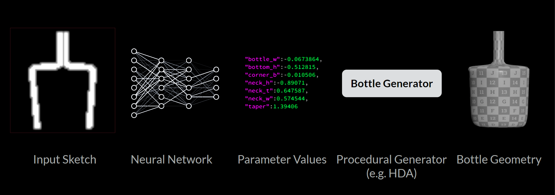
Doing so, we avoid all sorts of pitfalls and pain trying to predict geometry. The architecture comes with different pros and cons, which I will explain later. However, most of them are rather desirable, such as having clear constraints on what the model can output and not being too limited by the small resolution of the canvas:

• no matter what input is given the generator will always generate a somewhat sensible result
• the generator can create model details, that don’t need to be reflected in the input drawing

In this case we use compiled block for convenience and reusability reasons. That way we can run the setup in multiple locations while still being able to edit the functionality live. In general this could be an HDA.

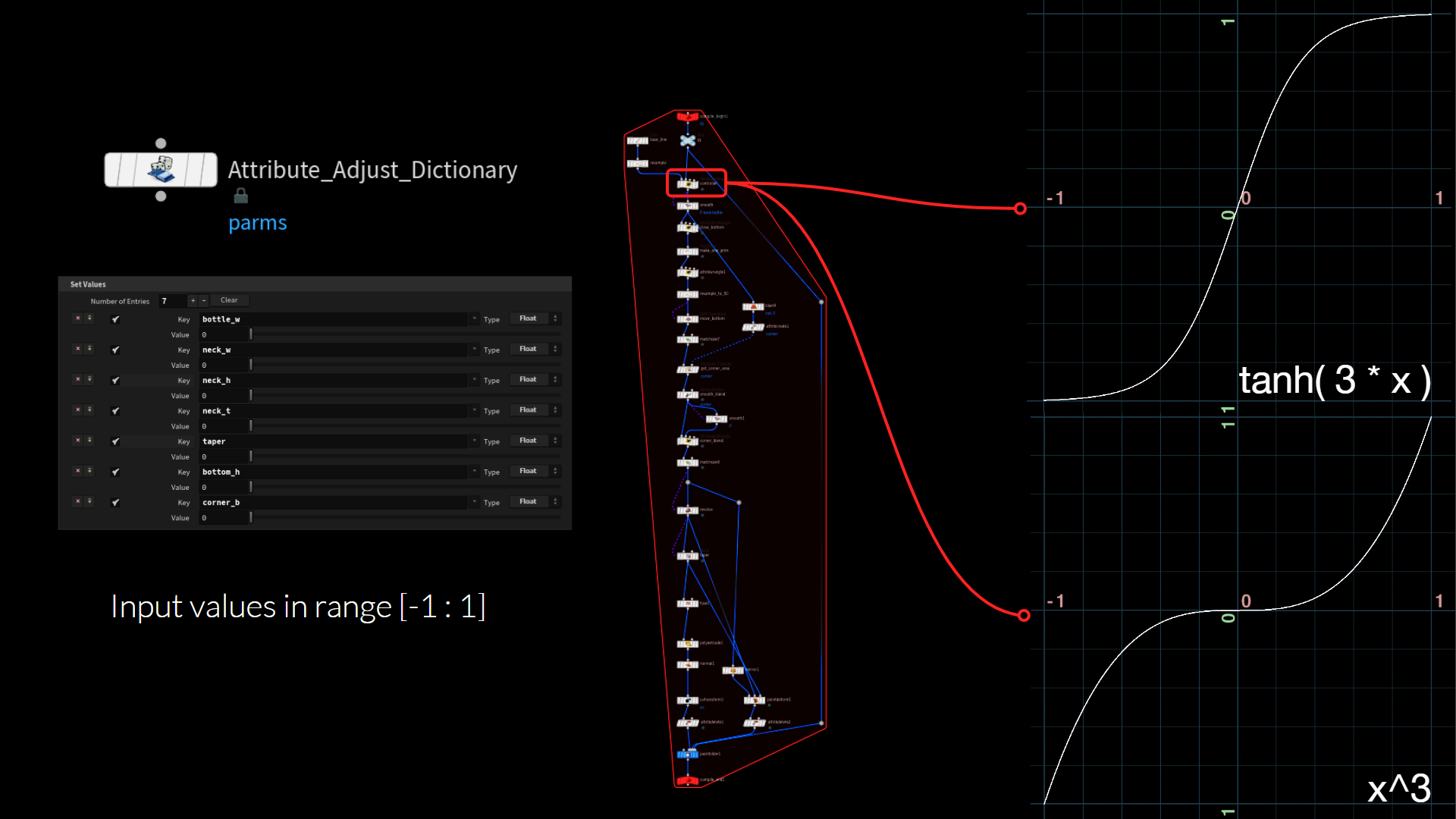
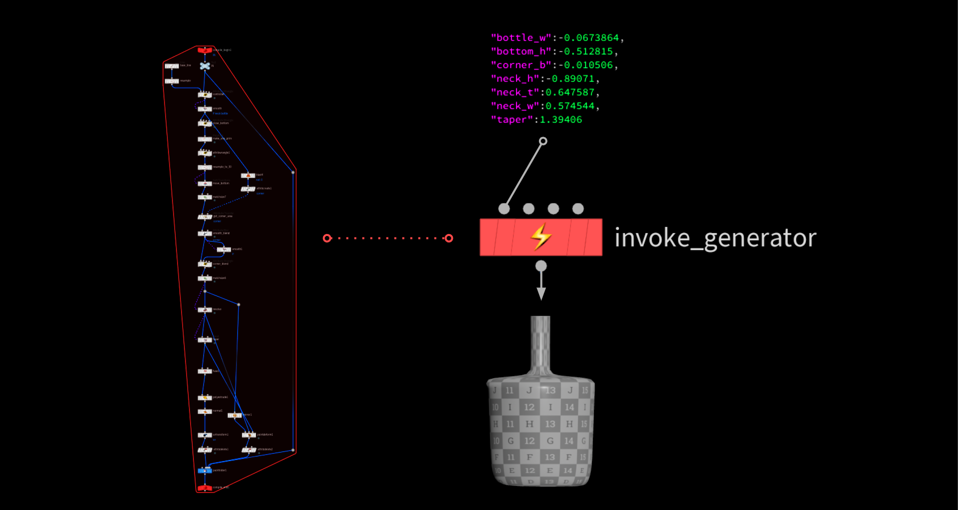
We control the parameters by storing them in a dictionary attribute that gets read inside the block before distributing the values to the correct nodes inside.

We want to avoid vastly different parameter value ranges to make training easier. All values are input in a -1 to 1 range which is a good normalization and fits the tanh() activation function that is used inside the network.

The parameter input values are remapped using sigmoid and cubic functions to control the distribution of random values when randomizing the generator later. The cubic function tends to cluster more values around zero, while the sigmoid function pushes more values toward the extremes of -1 and 1.

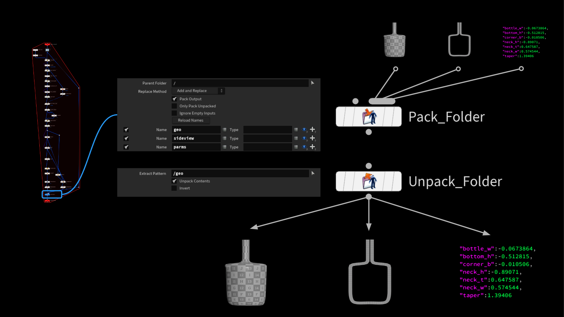
Another fun thing that is underrated is pack and unpack folders, which were originally introduced as part of the APEX/Character workflow. They are really useful to store different geometry streams in one and splitting  them apart again later based on their folder name. It’s really convenient and basically let’s you create a on the fly directory structure on your geometry.

Compared to the ML Groom Deformer demo, where the data generation is automated using TOPs, this time everything runs in a simple for each loop. This makes more sense because each example only takes a second or less to generate and spinning up entire Houdini instances in TOPs would create a bottle neck. Depending on the generation time and amount of examples needed it might make sense to implement a mix of both approaches:

Generate a bunch of examples in one workitem, but have multiple instances run at same time

Because the generator is just the compiled block we need to randomize the input dictionary. This is a super simple detail expression that randomizes each value based on the current iteration. Make sure to give a different offset/seed to each otherwise we get the same value in each parameter.

The invoke compiled block SOP then runs the generator and spits out our merged geometries, which we can access using the unpack folder SOP as mentioned above. The rest is just some data wrangling and rasterizing the outline on the image plane before storing it together with the parameter value list as a ml example.

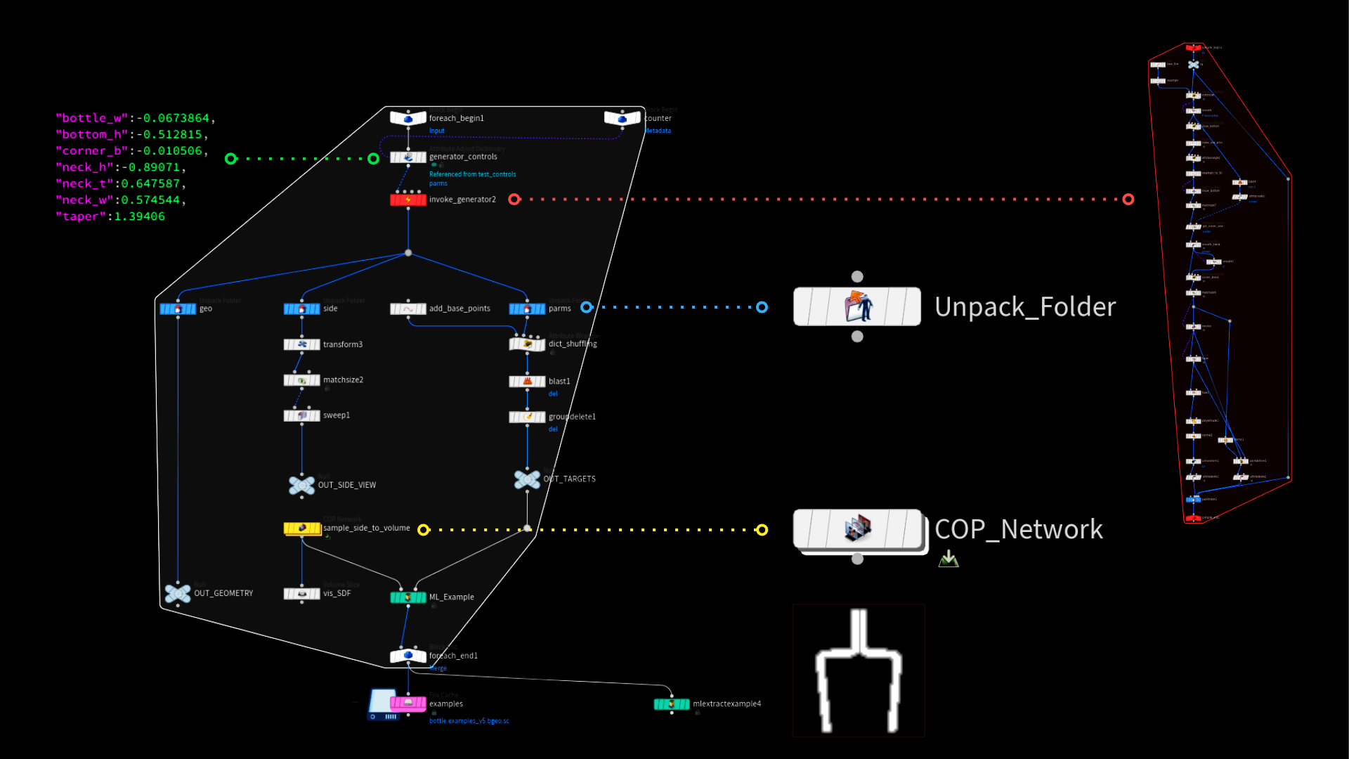
We use that loop to generate 10,000 examples and store those on disk.

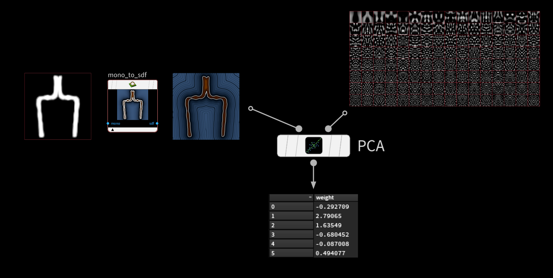
In the ML Groom Deformer project we used PCA to compress all the displacement samples into a smaller subspace, which allowed us to only store the weights for each example and not the whole geometry. We can do the same with our input images this time. Storing a 64x64 px image would mean feeding the neural network an array of 4096 float values. We can compress the image space of the 10.000 examples into much fewer components.

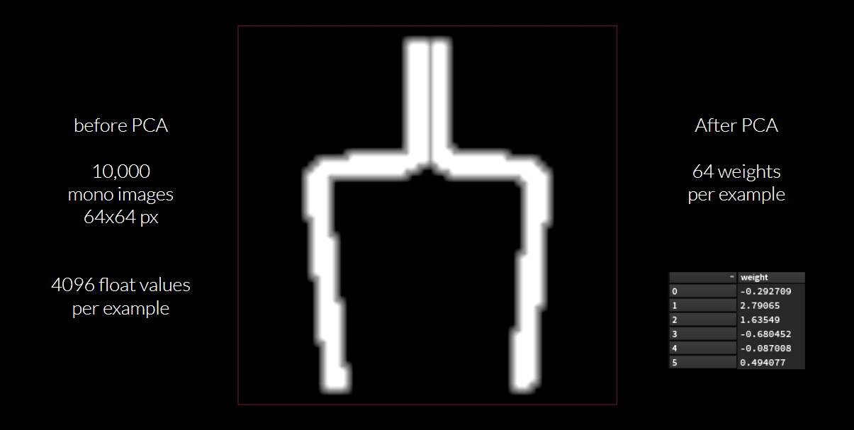
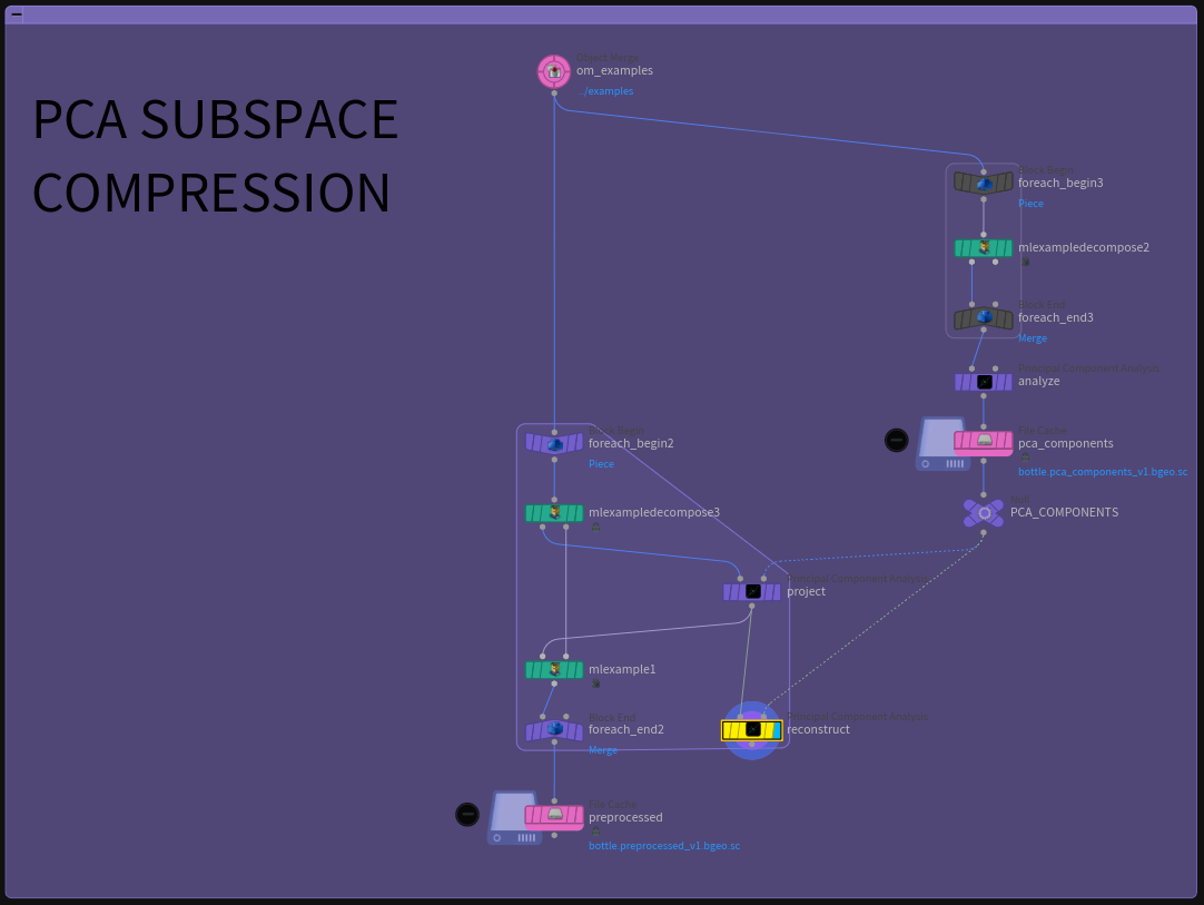
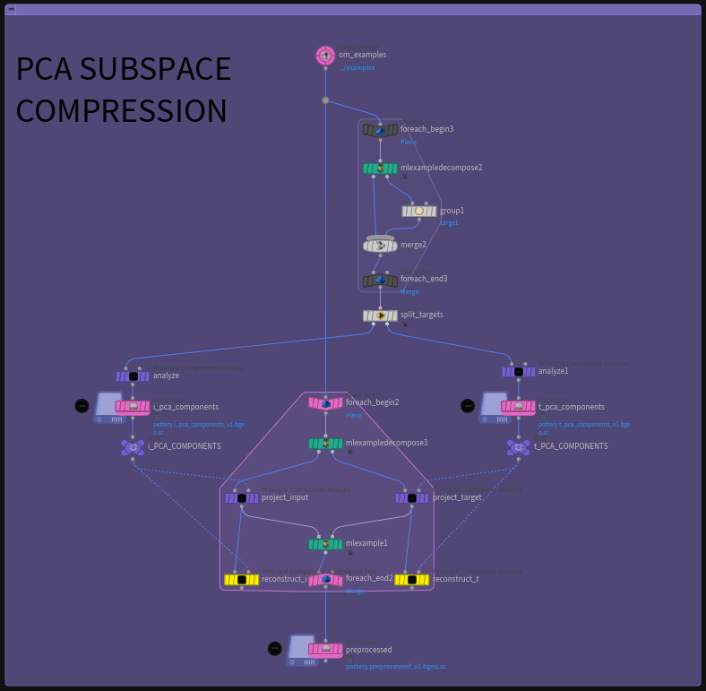
The setup looks something like this:

• on the right we unpack each input image and then analyze them using PCA
• then we can loop through each example and project each image into the subspace to get the weights
• We then replace the image volume in the example with only the weights (ml_example_decompose & ml_example SOPs)

When reconstructing (yellow node) the input image above we get something like this:

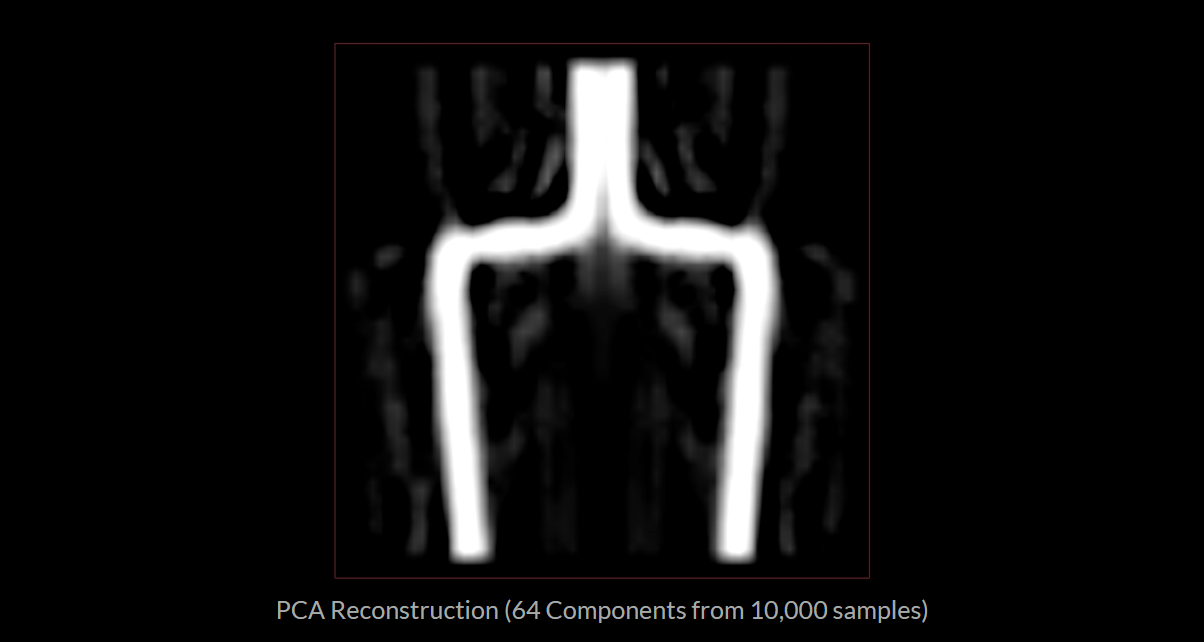
Which is kind of meh. We can make out the bottle shape but we get all of that unwanted wavy, noise like ghosting around it. Increasing the components surprisingly doesn’t help too much to improve the reconstruction.

What helps a lot is converting the black and white mask into an SDF using the new COPs SDF tools. That way we don’t have to deal with only 0 or 1 values and have a smooth gradual falloff around the bottle outline.

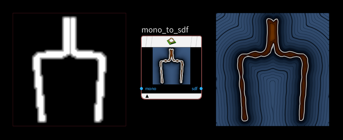
When reconstructing the SDF from a few components we get a near perfect result.

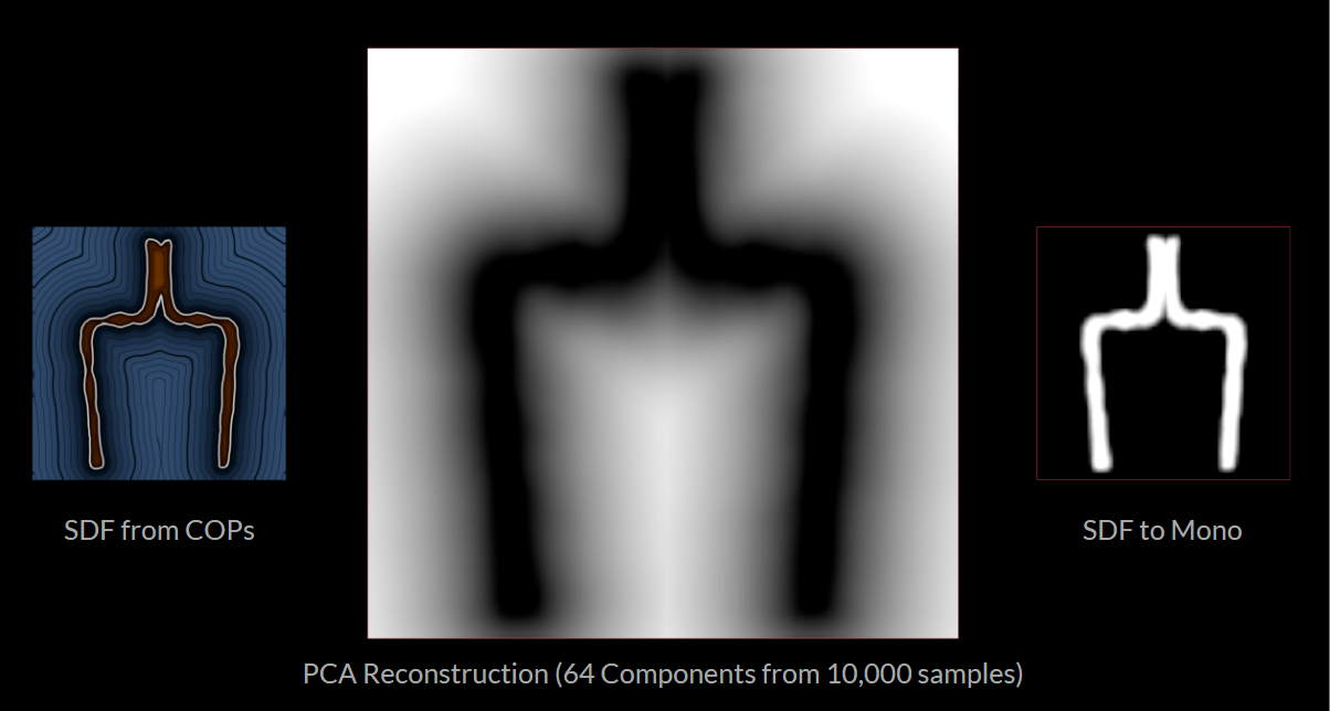
In that case 64 components were enough, because there was a lot of overlap in the input data. Even 32 looked fine, when testing, which is a crazy compression compared to the 10k input images.

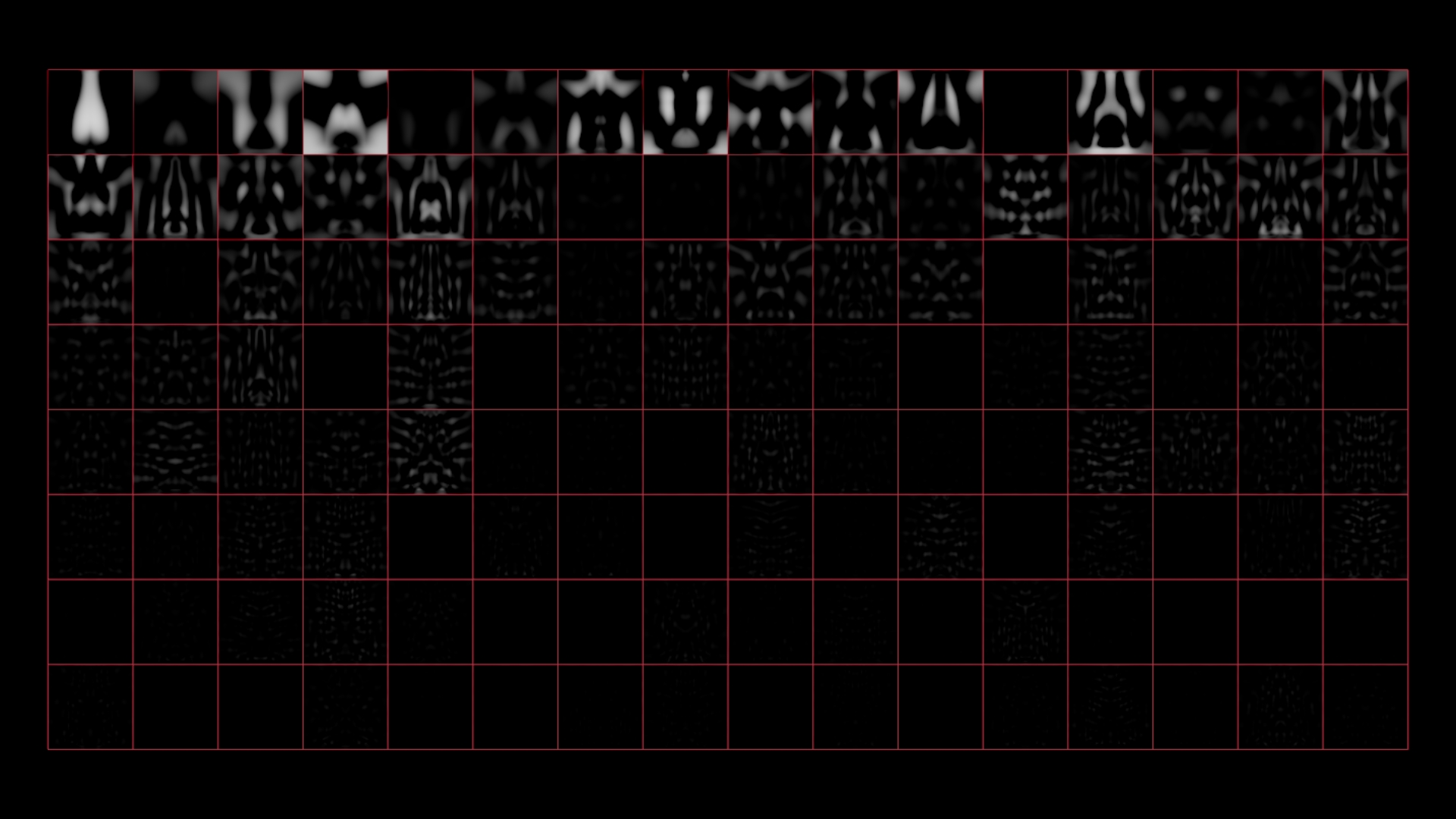
A really cool side effect of PCAing our images is that we can really visualize what each component looks like:

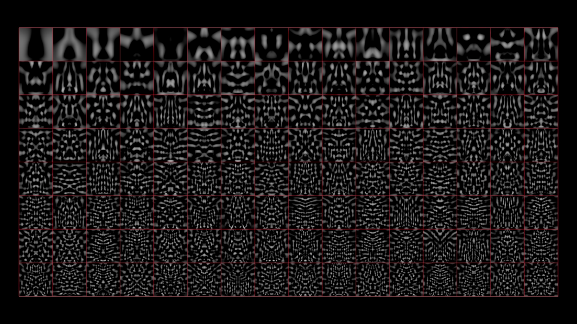
Because the components are ordered based on importance we can really see how much actual information each component stores before they gradually become less and less influential on the reconstruction. In the top left we can still make out the bottle shape, while in the bottom right it almost looks like noise.

Almost!

They kind of resemble Chladni Patterns. And that somewhat make sense. While Chladni Patterns are linear combinations of periodic functions our PCA components are linear combinations of all the bottle outline SDFs we provided PCA to analyze. This isn’t useful but I thought a pretty cool analogy and cross reference.

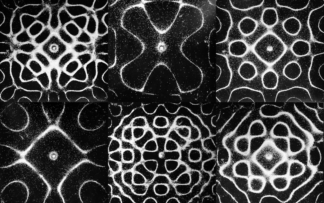
Source: List of Physical Visualizations; Dragicevic, Pierre and Jansen, Yvonne; 2012; https://dataphys.org/list/chladni-plates/

Having access to visually nice and somewhat sensible components also allows us to visualize how they should be weighted to reconstruct a given input.

Say a user draws the following shape(,which gets converted into an sdf under the hood). 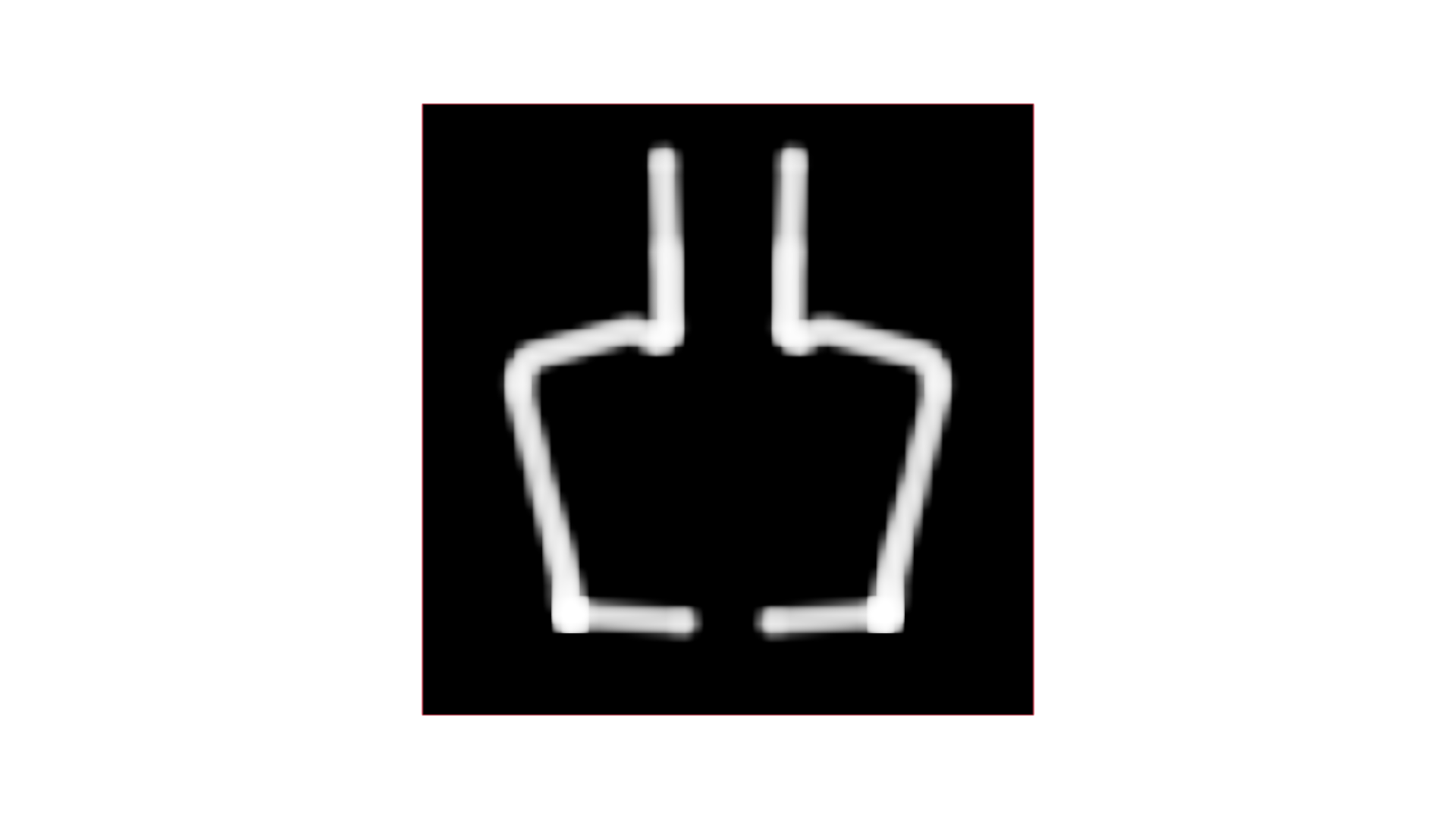Feeding this drawing together with the precomputed subspace components into the PCA SOP gives us the corresponding weights. If we apply those weights to their component counterparts we can really see which components make up the final reconstruction.

Adding them all together gives us the reconstructed SDF… which looks correct. Yey!

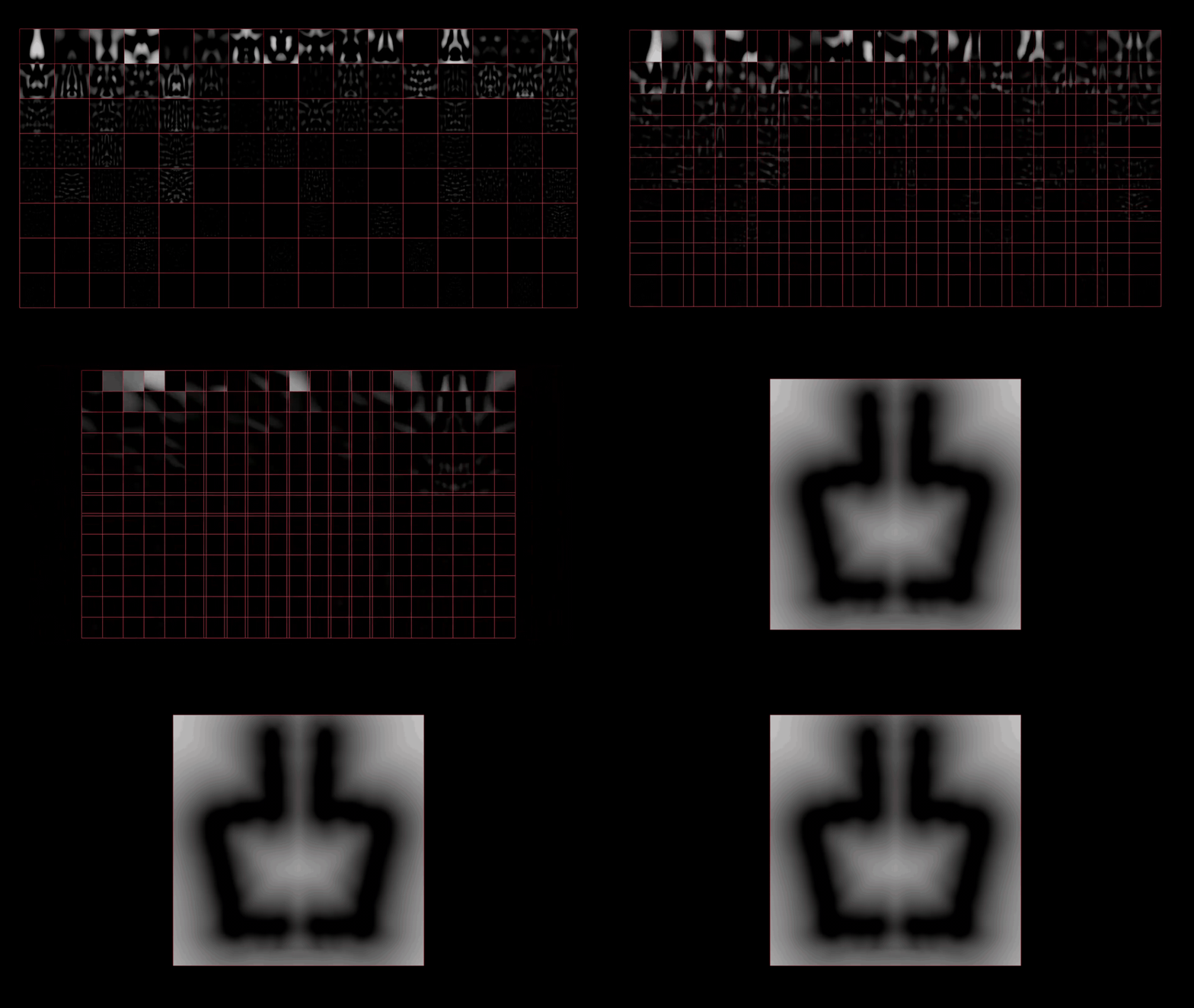
To recap: this working well with so few weights allows us to map from 64 input values (PCA weights) instead of 4096 float values to the 8 generator parameters.

This is all the data we have now:

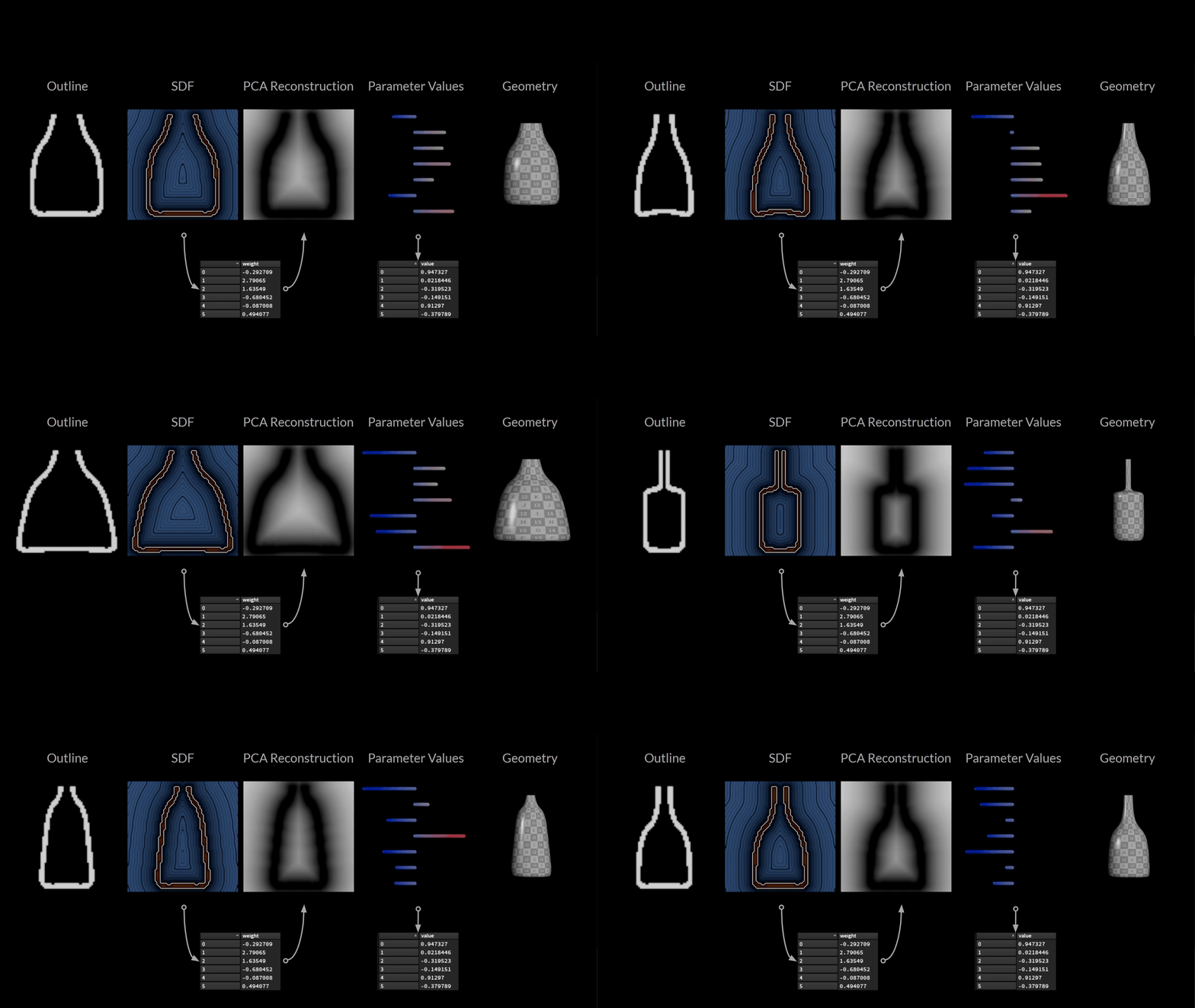
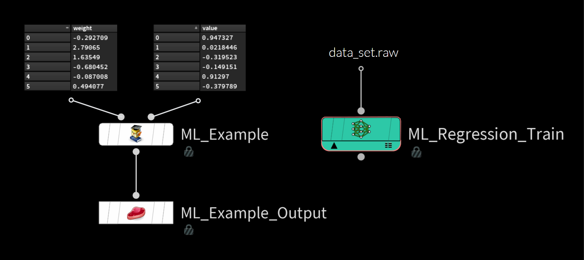
Our training examples are just two value lists:

• input: weights that describe the bottle outline image in the PCA subspace
• target: parameter values that describe the bottle shape

We store those on disk as a data_set.raw file using the ML Examples Output SOP and load it in the ML Regression Train TOP.

Once the data set is prepared and stored on disk as .raw file the rest is pretty straight forward.

The following paragraphs are copied 1:1 from the ML Groom Deformer project page.

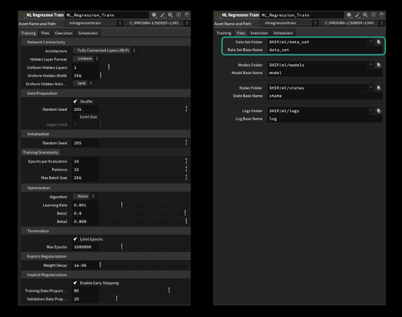
We can control all the parameters of the network (called hyperparameters for some obscure ml reason).

The most important ones are:

• Uniform Hidden Layers (how big is our network in width)
• Uniform Hidden Width (how many “neurons” each layer has)
• Batch Size (how many examples to look at before adjusting the weights > average)
• Learning Rate (how big the steps are the model takes towards the goal / think jumping down mountain or walking carefully)

To start training something we only need to make sure to specify the correct directory and name of our dataset on the files tab. By default this should be correct though. Be careful: Only specify the filename without the extension. It won’t run if we add the .raw. (last tested in H20.5.370)

Having all those parameters available on the node in TOPs opens the door to do some wedging! This is common practice and is usually called hyperparameter tuning. We could run multiple experiments to find the right combination of parameters that give we the best performing model. The parameters I mentioned above are a good place to start wedging. For the groom deformation example here I only wedged the amount of layers and the size of each layer.

As usual we need to perform all the steps of our data generation to get the input to the right shape. So we mirror the image to make sure it’s symmetrical and avoid introducing error on the user side. We then convert it to an SDF using the new mono_to_sdf COP node. We let PCA project those weights into our subspace and calculate the weights of the input.

We can then take those weights and feed them into inference SOP to let our model predict the correct parameters.

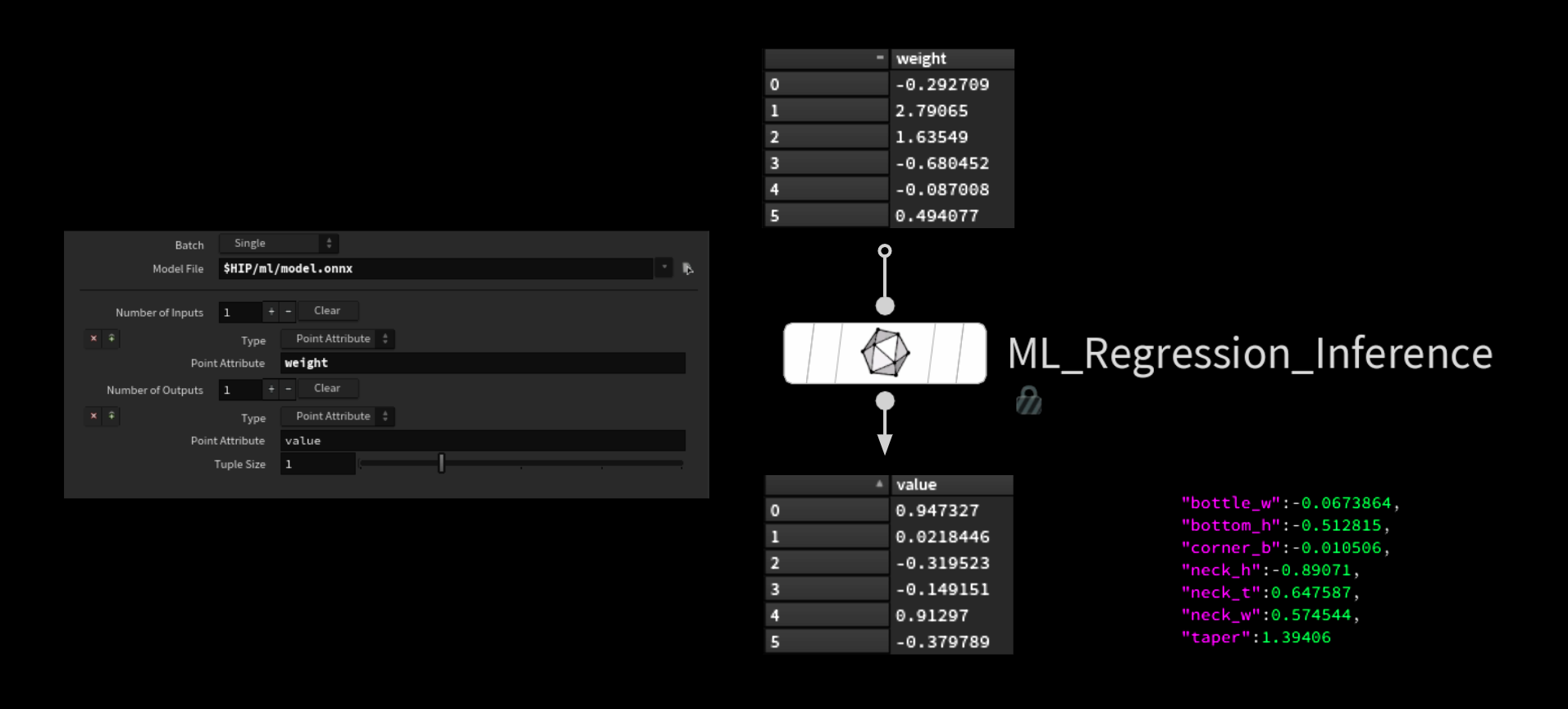
We turn the resulting value list into a dictionary and send it into the generator, which creates the corresponding bottle geometry.

// point wrangle (creating the dict)

1
2
3
4
5

dict parms = detail(1, "parms", 0); // input one is a template dict I read from disk
string keys[] = keys(parms);
dict newparms;
newparms[keys[@ptnum]] = @value;
setdetailattrib(0, "parms", newparms, "append");

The whole inference step is pretty fast and runs in realtime. The bottle neck here is the geometry generation step. When we hook the system up to a very involved HDA that e.g. builds ships instead of simple bottles we will run into performance problems. Might be worth having 2 different HDAs in that case:

1. to generate the silhouette and quickly iterate on broad shapes
2. to add detail and refine the shape in procedural ways that aren’t captured in the low res drawing canvas anyways

Combine that with some procedural COPs texture setup and we get something that looks much more involved than actually is!

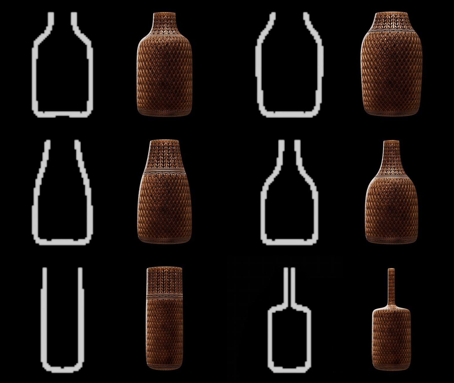Source: Texture Setup was created by Dixi Wen

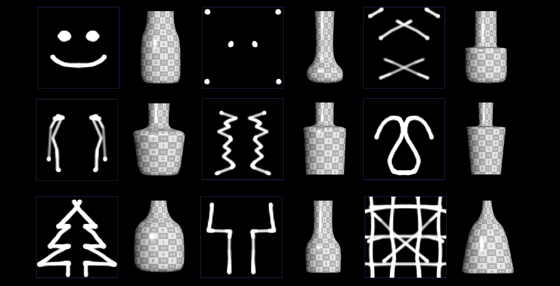
After showing this to my colleagues, they pretty much instantly started drawing random shit, which the generator can’t create, due to architectural constraints.

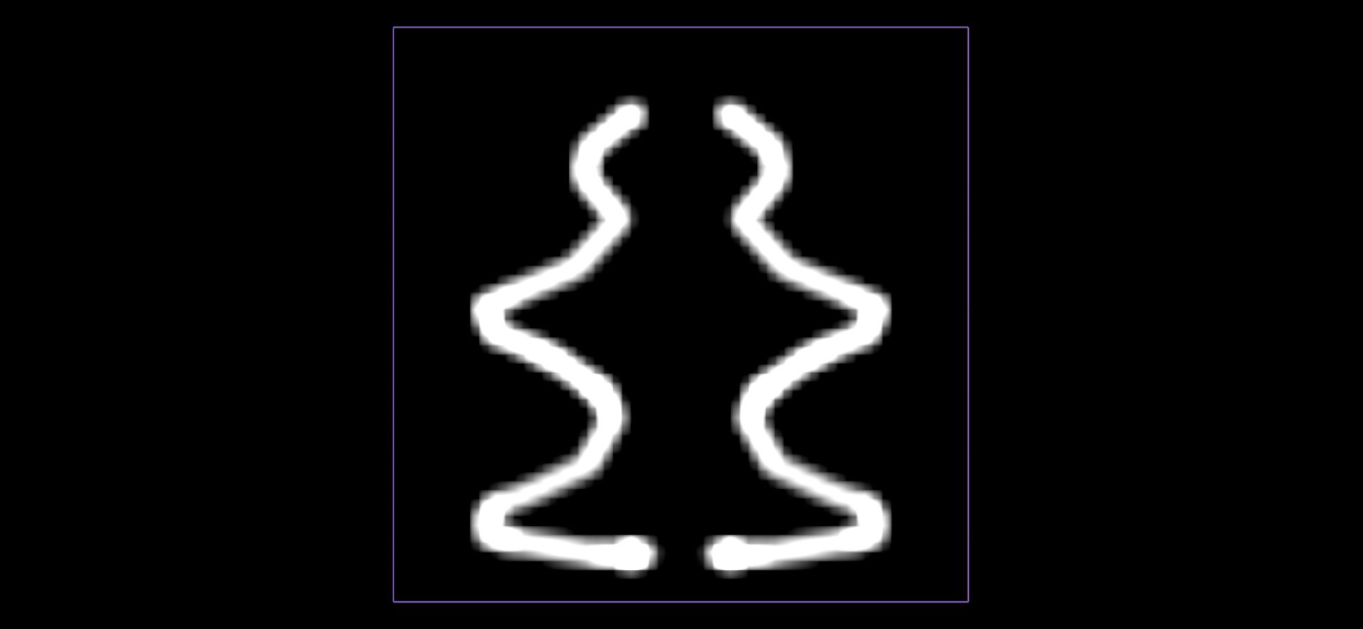
This can be a downside or a benefit. We will always receive a somewhat sensible output no matter what the input was. The output is constrained by what the generator can create.

Remember how SDFs compress really well with PCA? What if instead of learning to predict the parameters we try to predict a full 3d SDF?

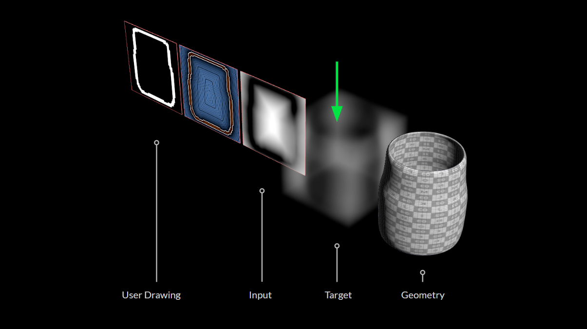
Just like before we PCA compress the inputs. For this approach however, we also do it for the outputs:

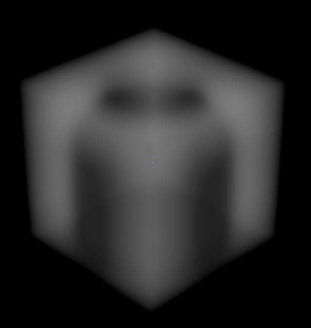
The 3D reconstruction looks like a fog volume:

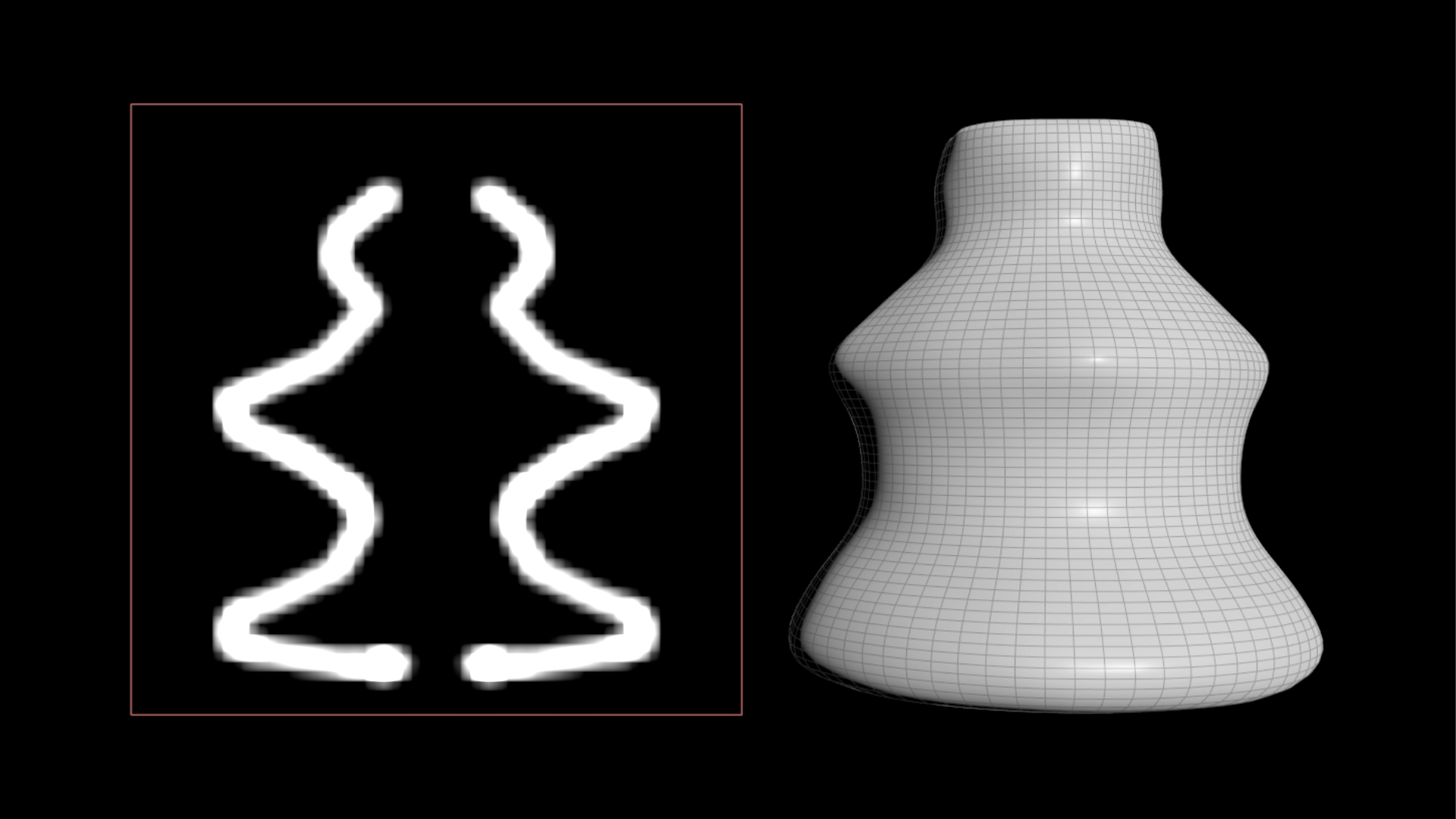
After converting it and cleaning it up a bit using vdb meshing techniques and then projecting clean uv’ed geometry onto it we get our bottle.

The main downside of this approach is that we need 2 generators. One to generate our training data and one that turns SDFs into usable geometry with good topology and uvs. That is also the most constraining part. Not every object can be converted so easily to good topology and a bottle is one of the easiest shapes.

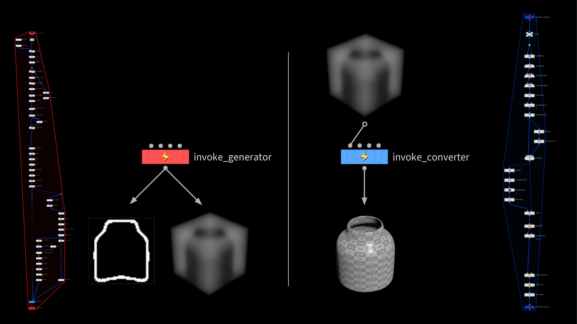
The left is the original generator, which is used to create the training data. Instead of storing the parameter values as targets it stores the fog SDF that is derived from the bottle geometry.

For the inputs we do the same (mirror, to SDF, PCA projection) thing we did before. We then run the outputs through PCA to reconstruct the 3D SDF based on the predicted weights.

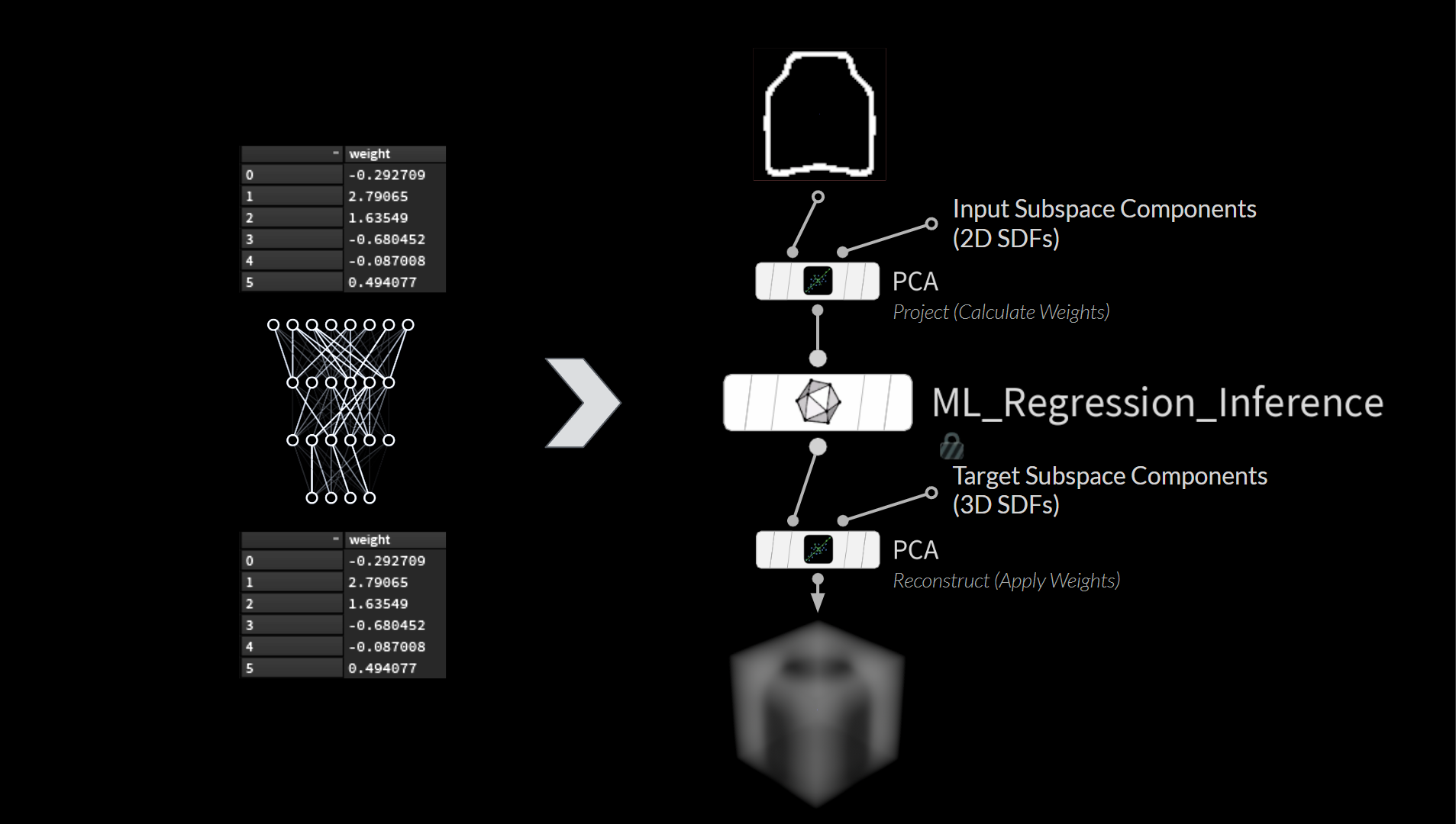
We feed this SDF into our second generator to turn it into clean geometry.

Accuracy and flexibility are much better, however speed suffers.

Because the second generator is the bottle neck the speed is much slower compared to the earlier version. However it’s outputs are much more flexible and we can draw “in between” shapes that didn’t even exist in the training data. There are still problems with sharp turns and overhangs that could be improved upon with other techniques or better training data.

The project builds on top of techniques learned, while building the ML Groom Deformer and extends concepts used for the Tower Sketcher project, which was part of my bachelor’s thesis.

The setup could be extended in the future through the use of CNNs and sparse network architectures to increase inference speed and improve accuracy.

Thanks to the amazing team at SideFX for all the help with this project!

Support on All Fronts: Fianna Wong ML Tools Developer: Michiel Hagedoorn COPs Bottle Texture Setup: Dixi Wen

sources / further reading:

• PCA Shenanigans and How to ML | Jakob Ringler | Houdini Horizon