Principal Component Analysis
“Principal component analysis is a versatile statistical method for reducing a cases-by-variables data table to its essential features, called principal components. Principal components are a few linear combinations of the original variables that maximally explain the variance of all the variables.”

Don’t Worry!
It’s just a method of summarizing some data typically used for statistics and machine learning applications.
I stole the following wine analogy from this excellent stack exchange explanation. I recommend reading this if you really want to understand it! The author goes into a lot more mathematical detail and explains it for different knowledge levels. I tried to explain just enough to make it useful for CG and not super confusing.
Imagine you have some wine bottles standing in front of you on the table. We can describe each wine by its colour, how dry or sweet it is, how strong it is, how old it is, and so on. We can compose a whole list of different characteristics for each wine.
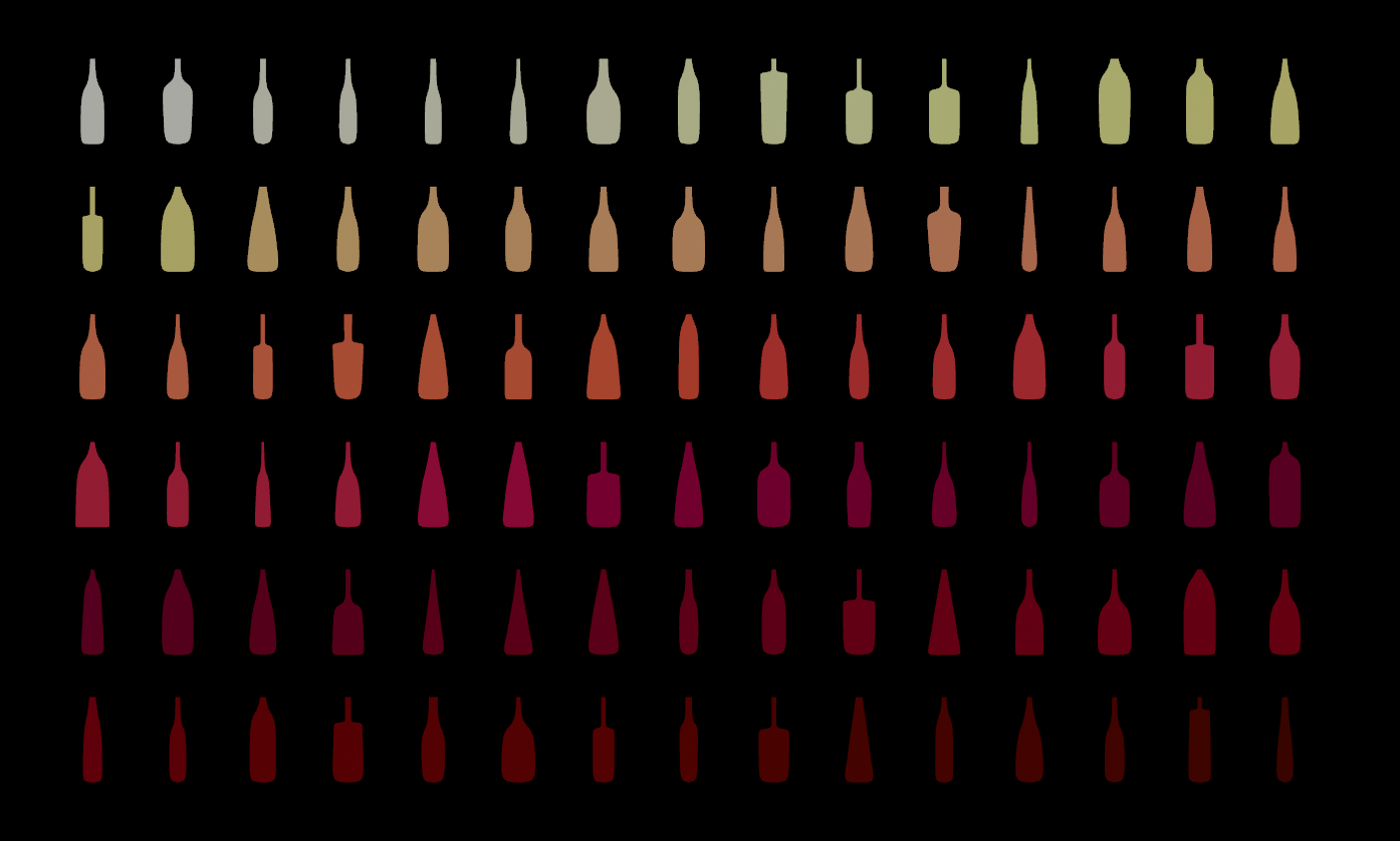
But many of them will measure related properties and so will be redundant. If so, we should be able to summarize each wine with fewer components! This is what PCA does. Instead of say 10 you may end up with 3 components that describe your data accurately enough Never 100% but close enough.

PCA is not selecting some characteristics and discarding the others. Instead, it constructs new characteristics called components that turn out to summarize our list of wines well. Those are linear combinations of the original data. One could look like this:
| |
In fact, PCA finds the best possible characteristics, the ones that summarize the list of wines as well as possible. Those components are ordered by importance, which comes in handy later.
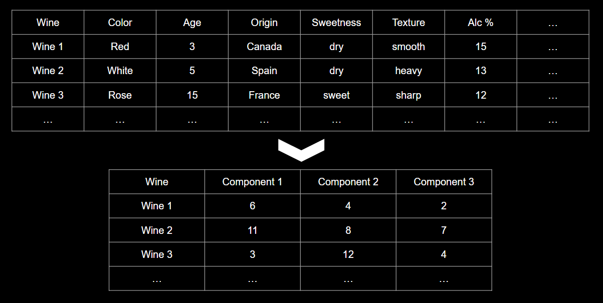
Note: all the data is generally in numerical form. So things like sweetness, texture etc would be encoded as a float range.
In 2d this could look something like this
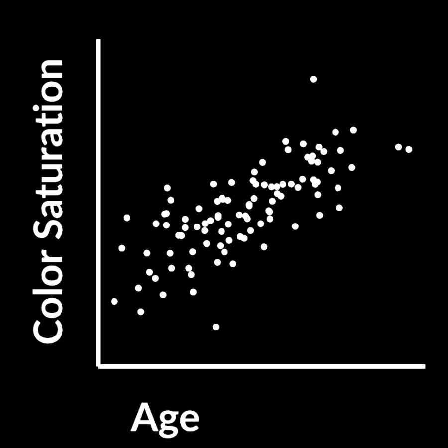
You have 2 axis, color and age and you have a scatter plot of different wines. This is of course not how wine works but lets just pretend that it gets more colorful over time.
If those two properties are related like that you can compress them because both store the same underlying information > time passed
The first PCA component for that data looks like this:
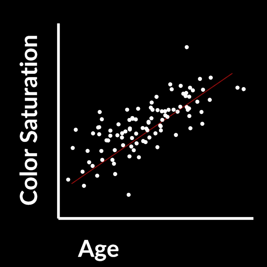
It’s the direction through your data where the most variance occurs. The longest distance essentially.
The second component would look like this:
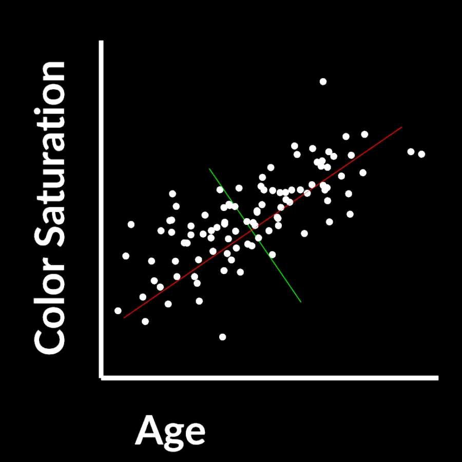
It is perpendicular to the first one and the second most important variance of the dataset.
What you can do then is project your original data samples onto the new components and calculate weights (how much of which component do you need) to reconstruct the original data point.
By doing that you create a new coordinate space where C1(red) is your new X axis and C2(green) is you new Y axis.
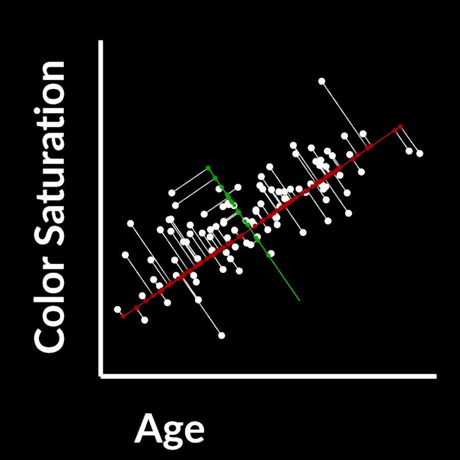
In 2d this isn’t very useful and doesn’t compress anything, but in highdimensional space you can compress your data a lot, while still maintaining most of the valuable information.
For general CG purposes it’s not too important to understand the math completely, but how to use it and what its good for.
So ..
# How is this useful for CG?
# General CG
# ML in Houdini
sources / further reading: